How Degrees of Freedom Survive Dimensional Reduction: Universal Clusters from Shielded Molecules to Species-Selective Traps

The claim under pressure

Dimensional reduction preserves a record of every coordinate that has been removed. In the two papers studied here, that record takes two different forms. Angular fluctuations around the attractive axis of a microwave-dressed dipolar potential contribute a distance-dependent zero-point energy, producing a short-range core in an effective one-dimensional potential. Transverse oscillator modes in a species-selective trap contribute virtual closed channels, producing energy-dependent one- and two-dimensional scattering amplitudes. Neither calculation amounts to deleting coordinates from a Hamiltonian. Each calculation integrates out motion and retains its low-energy consequences.

The distinction determines the meaning of every few-body result that follows. Tingting Shi, Haitian Wang, and Xiaoling Cui derive an effective one-dimensional description for microwave-shielded polar molecules in free three-dimensional space. They benchmark the reduction against exact three-dimensional two-molecule calculations and against a three-dimensional Born–Oppenheimer problem, then predict bound states of three identical molecules with an effective two-coordinate Hamiltonian. Tingting Shi and Xiaoling Cui solve a different reduction problem for heteronuclear atoms in quasi-one- and quasi-two-dimensional traps. They calculate the confined two-body $T$ matrix with center-of-mass coupling and finite Feshbach range, extract low-dimensional scattering parameters, and insert those parameters into Skorniakov–Ter-Martirosian equations for trimers and tetramers.

Both studies use the word universal. Here it means that a low-energy state can be specified without a microscopic chemical potential curve or an independent short-range few-body parameter. It does not mean parameter-free. The molecular problem retains the dipolar length, microwave coupling, detuning, and polarization. The atomic problem retains the three-dimensional scattering length, resonance range, mass ratio, confinement lengths, and frequency ratio. Universality compresses microscopic information into a controlled set of scales.

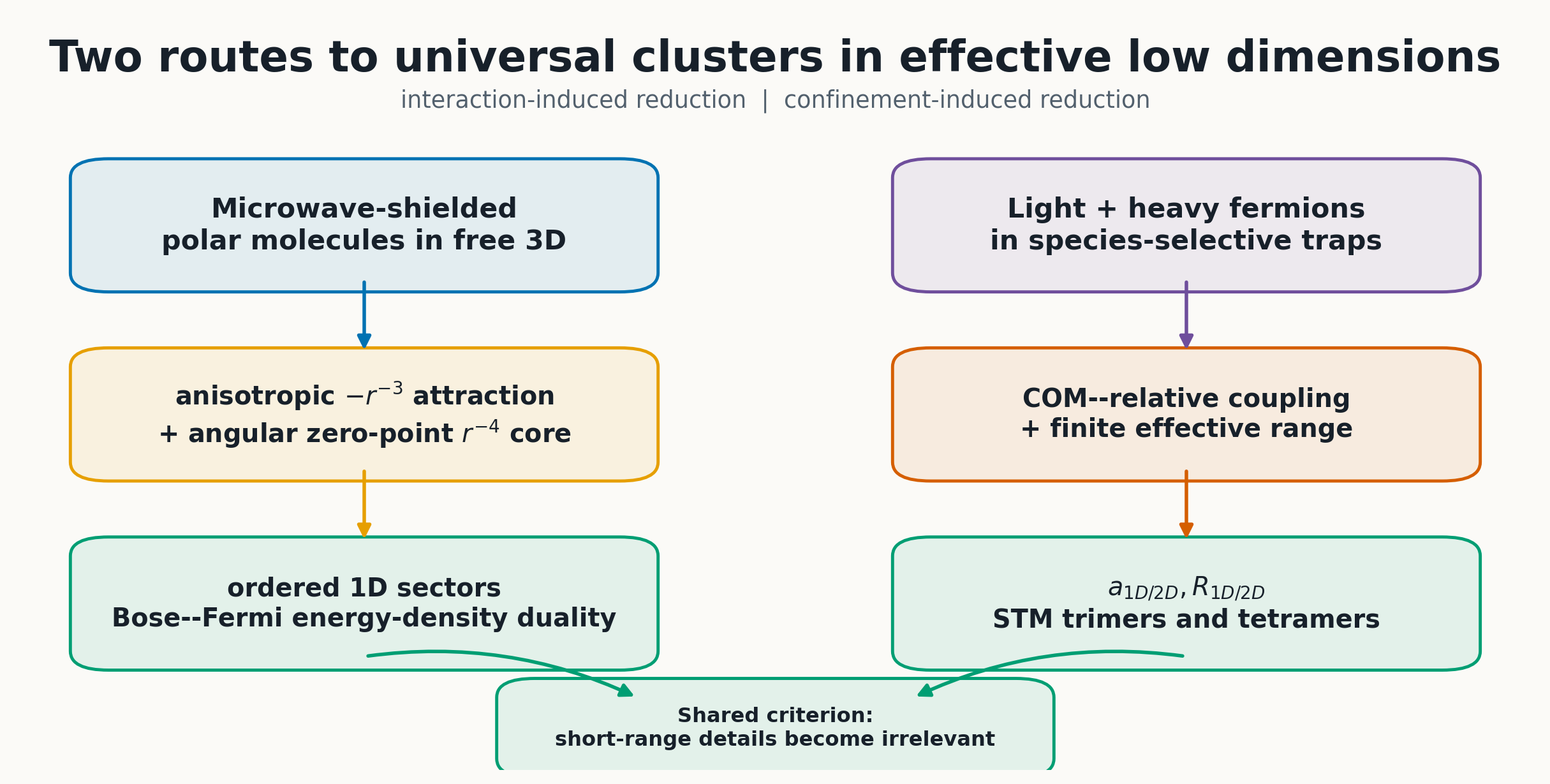
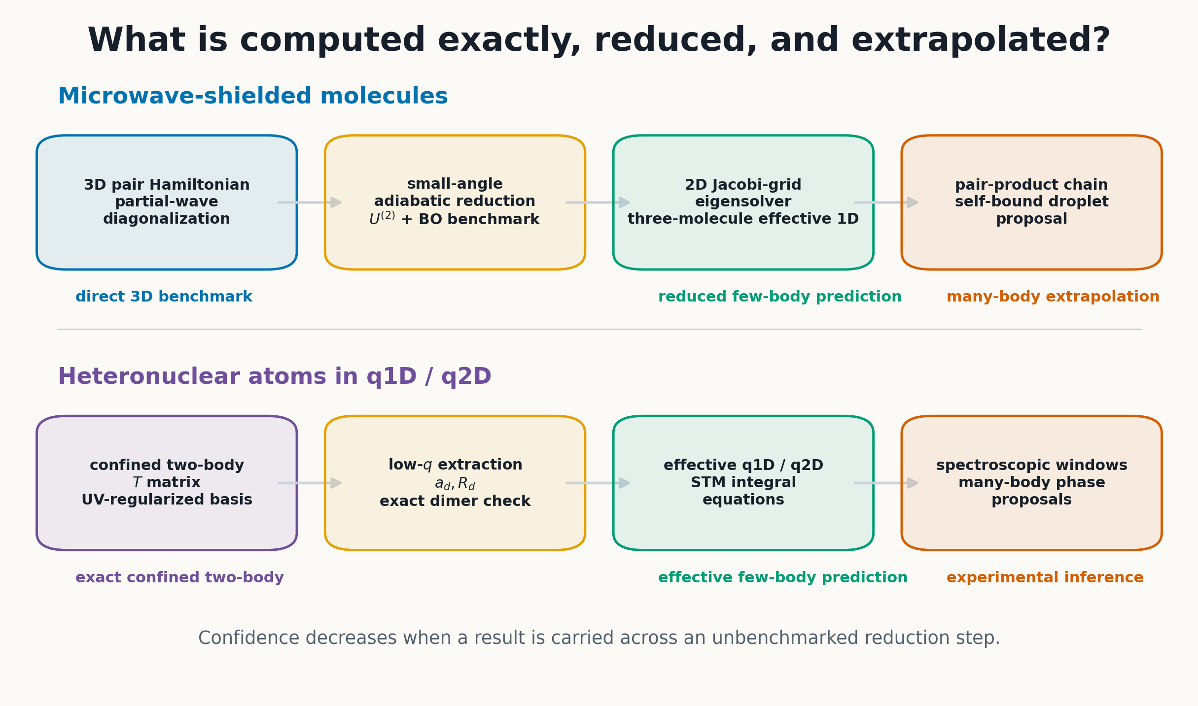
Figure 1. Two reductions with the same logical structure. The left branch converts angular motion in a three-dimensional anisotropic interaction into a one-dimensional potential. The right branch converts virtual transverse and center-of-mass excitations into low-dimensional scattering parameters. All diagrams in this entry were reconstructed from the published equations and data.

1. The objects, the versions, and the naming problem

The first source is Shi, Wang, and Cui, “Universal Bound States with Bose-Fermi Duality in Microwave-Shielded Ultracold Molecules”, read here in arXiv v4 dated January 28, 2026. Its elementary objects are diatomic molecules. A bound pair of those molecules contains four atoms and is called a tetratomic molecule; a bound state of three molecules contains six atoms and is called a hexatomic molecule. I will usually call them the two-molecule and three-molecule states because that language keeps the few-body counting visible.

The second source is Shi and Cui, “Effective scatterings and universal clusters of heteronuclear ultracold mixtures in quasi-low dimensions”, read in arXiv v1 dated June 3, 2026. Its elementary objects are atoms. One light atom with two identical heavy fermions is a trimer, while one light atom with three heavy fermions is a tetramer. The two papers therefore use the word tetramer at different microscopic levels.

The statistics also enter in different ways. The first paper compares identical bosonic and fermionic molecules and finds an emergent Girardeau-type mapping after the molecules become effectively impenetrable along one axis. The second paper keeps the heavy atoms fermionic from the start; antisymmetry appears explicitly in the exchange terms of the few-body integral equations. Conflating these mechanisms would hide the strongest conceptual result of each paper.

2. A scale test for any claim of effective low dimensionality

Suppose a system contains a slow energy scale $E_{\parallel }$ and an eliminated mode with gap ${\mathrm{\Delta }}_{\perp }$. A single-channel low-dimensional description needs a hierarchy such as

The hierarchy suppresses real occupation of the high-energy mode. Virtual occupation remains. If the interaction couples the low and high sectors, a Feshbach projection gives

where $P$ projects onto the low sector and $Q=1-P$. The second term depends on the discarded subspace. It can generate an induced repulsion, an energy-dependent coupling, a resonance, or a nonlocal operator. The low-dimensional model earns its status only after those contributions have been included and the result has been checked against the higher-dimensional problem.

The molecular paper realizes this formula in an adiabatic coordinate-space language. The slow coordinate is the separation along the attractive $y$ axis, while the fast coordinates are small angular excursions from that axis. The atomic paper realizes the same logic in scattering language. The open channel contains two transverse ground states; excited transverse and molecular center-of-mass levels form the closed sector. The first calculation retains a position-dependent zero-point energy. The second retains a threshold expansion of the $T$ matrix.

3. Experimental and theoretical setting

Microwave shielding has already changed the practical status of ultracold polar molecules. A near-resonant microwave field dresses rotational states and creates a long-range repulsive barrier that prevents colliding molecules from reaching chemically reactive separations. The original shielding proposal and coupled-channel analysis are given by Karman and Hutson in Physical Review Letters 121, 163401. Experiments have used the method to reach degenerate molecular gases, and field-linked resonances have provided an outer, anisotropic binding well on the safe side of the shield.

The most direct experimental precursor to the first paper is Chen and collaborators’ observation of ultracold field-linked tetratomic molecules. That experiment associated roughly $1.1\times {10}^3$ weakly bound NaK tetramers, measured a maximum free-space lifetime of $8(2)\mathrm{ms}$, and reconstructed an anisotropic momentum-space wavefunction. Those results establish that a long-range molecular complex can be prepared and imaged. They do not establish the three-molecule state predicted by Shi, Wang, and Cui.

Confinement-induced resonances provide the corresponding background for the second paper. Olshanii showed that a three-dimensional scattering length and a transverse oscillator length combine into an effective one-dimensional coupling in Physical Review Letters 81, 938. Bergeman, Moore, and Olshanii later demonstrated that the resonance can be viewed as a Feshbach crossing between an open transverse channel and a bound state in closed transverse modes in Physical Review Letters 91, 163201. Species-dependent confinement complicates that picture because the pair center of mass ceases to be a spectator.

The two 2026 papers push these established mechanisms into few-body territory. Their strongest contribution lies in the intermediate step between the microscopic Hamiltonian and the cluster spectrum. Control over this intermediate step separates benchmarked predictions from untested extrapolations.

---

4. Paper I: the dressed two-molecule interaction

4.1 Polarization convention and the long-range potential

Shi, Wang, and Cui use a microwave field

with ${\mathbf{e}}_{\pm }=\mp ({\mathbf{e}}_x\pm \mathrm{i}{\mathbf{e}}_y)$. Their main calculation takes $\xi =\pi /4$, which is linear polarization along $y$. They adopt an analytic dressed interaction previously derived for elliptic polarization and extrapolate it to this endpoint. At relative detuning ${\delta }_r=|\delta |/\mathrm{\Omega }=0.2$, the potential is

where

The angular factors expose the geometry immediately. Along $y$, one has $\theta =\pi /2$ and $\varphi =\pm \pi /2$, so the $C_3$ term becomes $-4C_3/r^3$. Along either $x$ or $z$, it becomes $+2C_3/r^3$. The explicit $C_6$ term vanishes on all three Cartesian axes and is repulsive in generic directions. The attractive channel is therefore a narrow valley surrounded by three-dimensional repulsion.

The authors define a dipolar length using the coefficient convention of this dressed potential,

then use $l_u=l_d/20$ and $E_u={\hslash }^2/(m{l}_u^2)$ as numerical units. They quote $l_d/({10}^4{a}_0)\simeq 1.1,2.6,8.3$ for NaK, NaRb, and NaCs. For NaK, $l_u\simeq 550a_0$, and a microwave coupling $\mathrm{\Omega }=2\pi \times 10\mathrm{MHz}$ corresponds to $\hslash \mathrm{\Omega }/E_u\simeq 52$.

The choice $\xi =\pi /4$ maximizes the single-axis attraction and makes the dimensional reduction unusually clean. It also sits at the least circular end of the polarization family. Coupled-channel shielding calculations with imperfect circular polarization show that increased ellipticity can reduce shielding efficiency. The first paper acknowledges this tension: smaller $\xi$ should improve loss suppression and add a direct $r^{-6}$ shielding core, while producing shallower states and eventually destroying the one-dimensional geometry.

4.2 The small-angle expansion

Choose either attractive direction ${\varphi }_0=\pm \pi /2$ and write

The supplemental material expands the potential to quadratic order:

The angular part of the kinetic energy contributes

At fixed $r$, the two angular coordinates form independent harmonic oscillators. Their combined levels are

The factor $r^{-2}$ in the angular kinetic energy matters. A $C_3/r^3$ angular curvature gives a zero-point scale $r^{-5/2}$, while a $C_6/r^6$ curvature gives $r^{-4}$. The latter diverges more rapidly than the attractive $r^{-3}$ channel and blocks access to the origin.

The expansion drops a term proportional to $\delta \theta {\partial }_{\delta \theta }$ from the spherical kinetic operator. The supplement argues that its ground-state expectation remains of constant order, while $⟨{\partial }_{\delta \theta }^2⟩$ grows as $1/r^2$ at short distance. The omission follows from power counting; no exact cancellation removes the term. Higher angular orders should matter first near the emergence of a broad state and when the polarization becomes less strongly one-dimensional.

4.3 Adiabatic separation and the effective potential

The authors write the relative wavefunction in an adiabatic basis,

where $y=r\sin {\varphi }_0$ labels the signed coordinate along the attractive axis. They retain the lowest angular channel and neglect derivative couplings between different $\nu$. The radial envelope then obeys

with

The approximation contains two separate assumptions. The angular wavefunction must remain localized near $y$, and transitions between adiabatic angular channels must remain weak. A small angular width supports the first condition. A large gap relative to the longitudinal kinetic matrix elements supports the second. The paper tests the combined approximation against exact three-dimensional states rather than estimating every nonadiabatic matrix element independently.

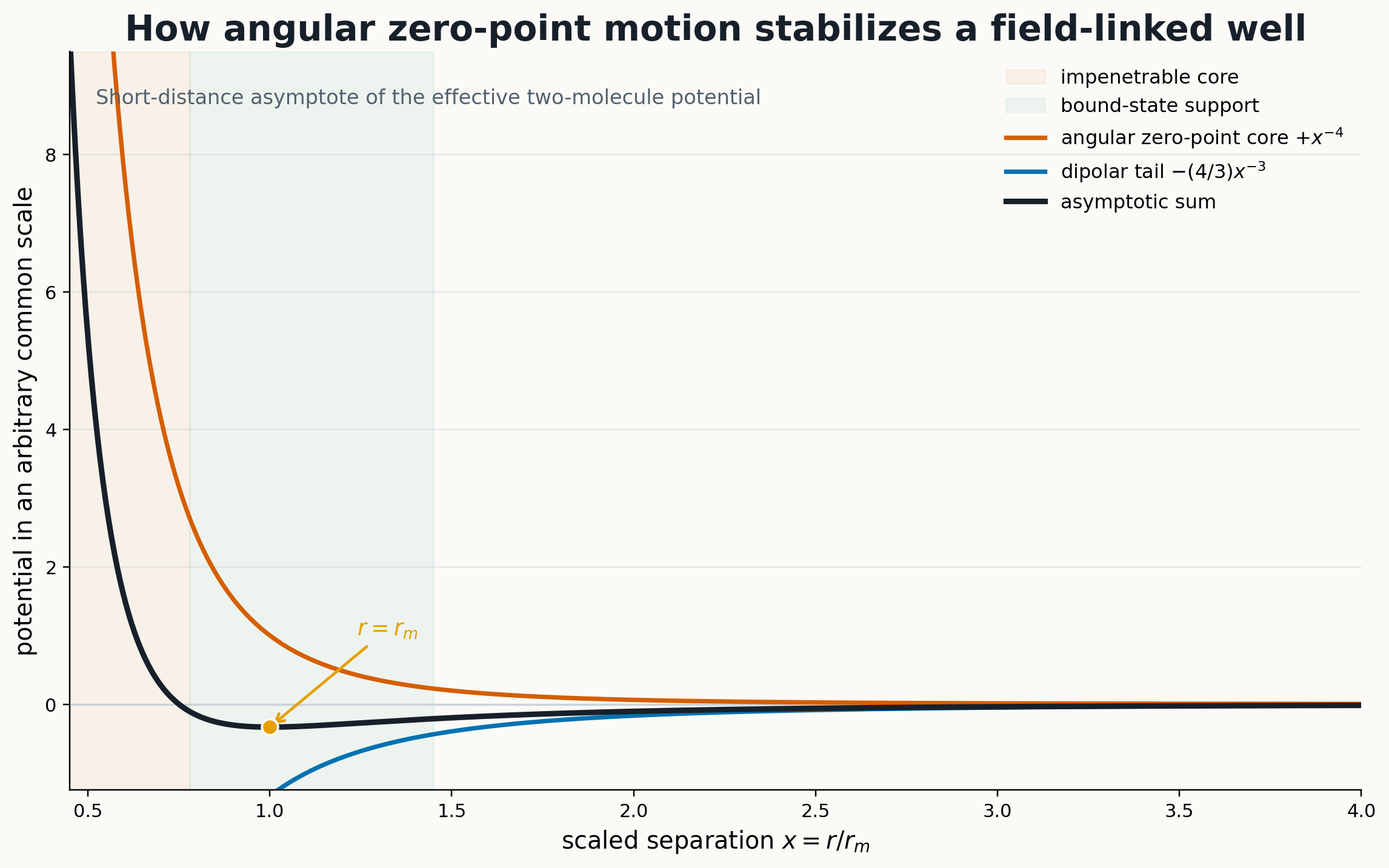
At short distance, the $C_6$ term inside the square root dominates:

Setting the derivative of this asymptote to zero gives

For ${\delta }_r=0.2$, the detuning factor differs from unity by roughly one percent, leading to the quoted estimate $r_m\simeq 4\sqrt{2},l_{\mathrm{\Omega }}$. The NaK example at $10\mathrm{MHz}$ gives $r_m=428a_0$. The state lives well outside chemical length scales and well inside the large dressed dipolar length.

Figure 2. Short-distance power counting for the effective two-molecule potential. The coefficients have been rescaled so that the asymptotic minimum lies at $r/r_m=1$. The plot shows the mechanism, not a fit to a specific molecular species. The full calculation uses the complete square root in $U^{(2)}$.

4.4 What the exact three-dimensional calculation contains

The two-molecule benchmark diagonalizes

in the basis

Bosonic exchange keeps even $\ell$; fermionic exchange keeps odd $\ell$. The microwave potential couples many $(\ell ,m)$ channels, so the two statistics generate different expansion coefficients even when their final probability densities become nearly indistinguishable. Any numerical reconstruction needs cutoffs in momentum, radial extent, $\ell$, and $m$. The public data do not include the convergence tables or assembly code for those cutoffs.

The exact spectrum contains two low levels that enter the bound sector one by one as $\mathrm{\Omega }$ increases. The effective one-dimensional energies are generally shallower near threshold because the quadratic angular approximation omits higher fluctuations. At stronger coupling, the one-dimensional energies track both exact parity sectors over a wide interval.

The supplement defines a signed one-dimensional reduction of the exact wavefunction,

and compares it with $F_0(y)$. Their overlap exceeds $97\mathrm{\%}$ once $\hslash \mathrm{\Omega }/E_u>10$. The boson-fermion energy mismatch is measured by

which falls below $5\mathrm{\%}$ for $\hslash \mathrm{\Omega }/E_u>2$. These two tests probe different errors. The overlap measures dimensional reduction; $\eta$ measures the onset of statistical duality.

4.5 The threshold region is genuinely three-dimensional

The exact bosonic state appears at a smaller critical $\mathrm{\Omega }$ than the exact fermionic state. Close to its emergence, the bosonic state follows the three-dimensional $s$-wave formula

and crosses threshold at $a_s\to \mathrm{\infty }$. The fermionic threshold state has $p$-wave character. The effective one-dimensional model cannot reproduce two different threshold laws because it gives the same impenetrable-channel spectrum to both statistics.

A near-threshold state extends far beyond the narrow attractive valley. It samples the full angular manifold and resolves the difference between even and odd partial waves. Increasing $\mathrm{\Omega }$ shrinks the bound state toward $r_m$, raises the barrier against exchange, and confines its probability to the axial valley. The effective one-dimensional description improves as the state becomes more deeply bound.

The supplement also identifies the only plausible Efimov window. Dipolar Efimov scaling would require $l_d\ll r\ll |a_s|$. For the molecular parameters used here, $|a_s|>l_d=20l_u$ occurs only in the narrow interval $\hslash \mathrm{\Omega }/E_u\in (0.5,1.5)$ around the $s$-wave resonance, where $|E_b^{(2)}|\lesssim 0.004E_u$. Any Efimov states in that interval would lie close to threshold and outside the compact universal-cluster regime centered near $r_m$.

5. Bose–Fermi duality in the molecular problem

An impenetrable one-dimensional core divides configuration space into ordered sectors. For $N$ particles, one sector is $y_1<y_2<\cdots <y_N$; the remaining $N!-1$ sectors follow by permutation. The wavefunction vanishes on every coincidence hyperplane $y_i=y_j$, so no continuous path exchanges two particles inside the low-energy manifold.

Given a symmetric solution ${\mathrm{\Psi }}_B$, the Girardeau mapping constructs an antisymmetric one,

The two states have the same energy and the same coordinate probability $|\mathrm{\Psi }{|}^2$. The density and the diagonal pair correlation

therefore coincide. The mapping changes the phase between ordered sectors. The one-body density matrix, momentum distribution, exchange response, and other off-diagonal observables can still distinguish the statistics. The exact three-dimensional states realize the mapping approximately because the core is high rather than mathematically infinite and because some transverse amplitude remains.

The shallow threshold states prevent a broad claim of statistical equivalence: their $s$- and $p$-wave emergence points differ. The paper establishes near equality of energies and spatial densities only in the compact, effectively one-dimensional coupling range. Exchange phases and non-diagonal observables retain the molecular statistics.

6. The three-body benchmark: Born–Oppenheimer geometry

The authors place two infinitely heavy molecules at $\pm \mathbf{R}/2$ and diagonalize the light-molecule Hamiltonian

Its eigenvalue defines a light-induced heavy-heavy potential $V_{\mathrm{BO}}(\mathbf{R})$. The calculation again uses the full three-dimensional $(k,\ell ,m)$ basis. It tests the reduction in a three-particle sector while avoiding the full six-dimensional motion of three equal masses.

For $\mathbf{R}\parallel y$, the exact spectrum contains two low branches. One places the light molecule between the two heavy molecules; the other places it outside them. At large $R$, either branch approaches a heavy-light dimer plus a distant heavy molecule. The leading shift can be reproduced by the expectation value of the distant interaction in a dimer state, because overlaps between dimer bases centered on opposite heavy molecules become negligible.

The inner behavior separates the branches. The inside configuration forces the light molecule toward both short-range angular cores as $R$ decreases, so its energy turns upward. The outside configuration can move away from both cores and continues downward, eventually saturating at the light-particle energy in approximately twice the single-center potential. When $\mathbf{R}$ points along $x$ or $z$, the potential is higher; the two orientations are symmetry-equivalent for the chosen dressed interaction.

The corresponding one-dimensional light-particle potential is

It reproduces the exact branches well for $\mathbf{R}\parallel y$ at the representative coupling $\hslash \mathrm{\Omega }/E_u=52$. The computed $V_{\mathrm{BO}}(R)$ shows no attractive $-1/R^2$ interval, supporting suppression of Efimov physics in the scanned compact-cluster regime. A finite-mass calculation near the narrow $s$-wave resonance would be needed for a broader exclusion.

7. Three identical molecules in the effective one-dimensional theory

7.1 Jacobi coordinates and four angular modes

For three equal masses, the paper introduces orthogonal Jacobi vectors

Their axial projections are $y_r$ and $y_{\rho }$. The three pair separations along $y$ are proportional to

Small deviations of $\mathbf{r}$ and $\mathit{\rho }$ produce four angular variables. The polar pair $(\delta {\theta }_r,\delta {\theta }_{\rho })$ and azimuthal pair $(\delta {\varphi }_r,\delta {\varphi }_{\rho })$ form two independent coupled-oscillator blocks. A generic block has the form

The supplement diagonalizes this quadratic form. Its ground energy can be written as

Applying this expression to both angular blocks produces $u^{(3)}(y_r,y_{\rho })$, the three-body zero-point surface. The final effective Hamiltonian is

The three coincidence lines divide the $(y_r,y_{\rho })$ plane into six wedges, one for each ordering of the molecules. $U^{(3)}$ is symmetric under reflection across those lines. Bosonic and fermionic states use symmetric and antisymmetric continuations across wedges, while their probability density within a wedge remains the same when the core suppresses tunneling.

7.2 Spectrum, wavefunction, and pair correlations

The authors discretize the two-dimensional Jacobi plane and diagonalize $H_{1\mathrm{D}}^{(3)}$. The two lowest three-molecule levels are deeper than the corresponding two-molecule levels. The ground-state binding exceeds twice the two-molecule binding, which rules out a picture of a bound dimer plus a passive spectator.

The pair correlation has peaks near $r_m$ and $2r_m$. The first peak counts nearest neighbors in a three-site chain. The second counts the two end molecules. In the pair-product approximation discussed below, the result follows analytically from

The first term places the two observed particles on one bond; the convolution places an unobserved molecule between them. The correlation function therefore resolves the chain geometry without assigning labels to identical particles.

7.3 Pair-additive approximation and the origin of extra binding

The paper compares the full zero-point surface with

Inside the ordered sector $y_1<y_2<y_3$, use $y_{12}$ and $y_{23}$. After removing the center of mass,

The mixed derivative appears because adjacent bond coordinates are not orthogonal. The supplement finds that this kinetic contribution is small for localized neighboring bond states. The direct interaction between molecules 1 and 3 supplies most of the negative correlation energy. At equilibrium it is approximately $-4C_3/(2r_m{)}^3$.

Using the two lowest dimer orbitals, the authors diagonalize a $3\times 3$ truncated basis built from

The ground state is dominated by the first product and has near-unit overlap with the full effective calculation. The first excited state resembles the symmetric combination in which either bond is excited. Its overlap exceeds $60\mathrm{\%}$ for $\hslash \mathrm{\Omega }/E_u\gtrsim 20$. The lower overlap flags stronger configuration mixing in the excited sector.

7.4 From three molecules to a chain

For $N$ ordered molecules, the proposed ground state is a product of neighboring bond orbitals. Treating each molecule as localized with spacing $r_m$, the non-nearest-neighbor dipolar correction is

At large $N$,

where $\zeta (3)-1\simeq 0.2020569$. The correction is extensive and negative. It supports a stable chain-like energy density within the localized-bond approximation.

It does not complete a thermodynamic proof of a self-bound droplet. Such a proof would require the full large-$N$ equation of state, a positive compressibility in the equilibrium phase, a surface-energy analysis, competing transverse configurations, and a lifetime longer than the equilibration time. The paper calls the proposed state an elongated crystalline self-bound droplet; the numerical evidence directly reaches three identical molecules and an analytic large-$N$ estimate.

8. Reconstructing the molecular calculation in code

The associated Figshare archive contains plot tables, two-dimensional potential matrices, wavefunction grids, Born–Oppenheimer curves, energies, and overlaps. It contains no source code. A reproduction therefore has to infer numerical choices from the equations and supplement.

8.1 Effective two-body solver

A minimal finite-difference solver is short:

import numpy as np
from scipy.sparse import diags
from scipy.sparse.linalg import eigsh

def U2(r, C3, C6, hbar, mass):
    angular_zpe = np.sqrt(
        (4 * hbar**2 / mass) * (6 * C3 / r**5 + 4 * C6 / r**8)
    )
    return -4 * C3 / r**3 + angular_zpe

def dimer_spectrum(r_min, r_max, points, C3, C6, hbar, mass):
    r = np.linspace(r_min, r_max, points)
    dr = r[1] - r[0]
    laplacian = diags(
        [np.ones(points - 1), -2 * np.ones(points), np.ones(points - 1)],
        [-1, 0, 1],
    ) / dr**2
    H = -(hbar**2 / mass) * laplacian + diags(U2(r, C3, C6, hbar, mass))
    energy, state = eigsh(H, k=4, which="SA")
    return r, energy, state

The short code omits the reliability tests. One must vary $r_{min}$, $r_{max}$, and the grid spacing independently; compare energy, rms radius, and contact suppression; and verify that the exponential tail dies before the box boundary. A mapped grid or finite-element basis will resolve the singular core more efficiently than a uniform mesh.

8.2 Exact partial-wave solver

The three-dimensional code should construct kinetic blocks diagonal in $(k,\ell ,m)$ and potential blocks

The angular integral can be cached as sparse tensors for the $r^{-3}$ and $r^{-6}$ structures. Scanning $\mathrm{\Omega }$ then changes $C_6$ without recomputing every quadrature. Even- and odd-$\ell$ bases generate the bosonic and fermionic sectors. A credible convergence table varies the radial box, the number of radial modes, ${\ell }_{max}$, and the retained $m$ range. The shallow state near resonance demands a much larger box than the compact state at $\hslash \mathrm{\Omega }/E_u=52$.

8.3 Three-body angular Hessian and Jacobi grid

For every $(y_r,y_{\rho })$ grid point, the program forms the two $2\times 2$ quadratic blocks for the $\theta$ and $\varphi$ fluctuations. Mass-weighted diagonalization gives four positive frequencies; their half-sum yields $u^{(3)}$. Points on a coincidence line require a boundary treatment because the effective potential diverges. Solving within one ordered wedge with Dirichlet conditions on its edges is cheaper and makes the Bose–Fermi mapping explicit.

The kinetic operator is a Kronecker sum on an orthogonal $(y_r,y_{\rho })$ grid. A sparse eigensolver returns the lowest states. The calculation should check symmetry under all three wedge reflections, normalization, grid refinement, box size, and stability of overlaps against the pair-additive basis. Negative eigenvalues of an angular Hessian would signal that the axial saddle is locally unstable and that the reduction has left its domain.

8.4 A test hierarchy

The implementation can be tested from the inside out. The analytic oscillator frequency checks the angular Hessian for two molecules. The $r^{-4}$ short-distance slope checks the effective potential. Exact one-dimensional dimer energies check the radial discretization. The published $97\mathrm{\%}$ overlap checks the three-dimensional reduction. Permutation symmetry checks the three-body surface. The two peaks of $G_2$ check coordinate transformations and normalization. Reproducing a plotted eigenvalue without these internal tests would leave several compensating errors undetected.

---

9. Paper II: the confined heteronuclear Hamiltonian

Shi and Cui start from two atoms with masses $m_h$ and $m_l$,

using $\hslash =1$. The bare coupling obeys

The divergent momentum sum is part of the definition of the zero-range interaction. It must cancel an equal divergence in the pair propagator. Treating $g$ as a finite grid parameter without this cancellation would make every extracted scattering length depend on the ultraviolet cutoff.

The narrow heteronuclear Feshbach resonances also require an energy-dependent inverse scattering length,

The positive parameter $R^{\ast }$ is related to the conventional effective range by a sign and normalization convention. The paper retains $R^{\ast }$ explicitly because its candidate Li–Cr and Li–K resonances have values of thousands of Bohr radii.

10. Center-of-mass coupling from species-selective confinement

Consider one confined coordinate. Define

The inverse transformation is

Substituting into the two harmonic traps gives

with

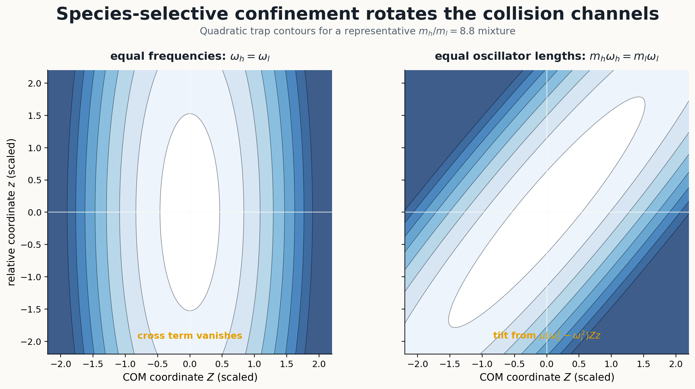
Equal trap frequencies remove the cross term. Equal oscillator lengths do not. The numerical examples set

so ${\omega }_h/{\omega }_l=m_l/m_h$. A mass-imbalanced pair then has strongly unequal frequencies and a tilted quadratic form in $(Z,z)$. The closed channels carry center-of-mass excitation as well as relative excitation.

Figure 3. The trap potential in center-of-mass and relative coordinates for a representative Li–Cr mass ratio. Equal frequencies produce aligned contours. Equal oscillator lengths, the choice used in the paper’s numerical examples, rotate the normal modes and couple collision energy to several molecular center-of-mass levels.

11. Quasi-two-dimensional scattering

11.1 Open channel and threshold form

In quasi-two dimensions, the $z$ coordinates are trapped and the relative in-plane coordinate $\mathit{\rho }$ is free. The incident state is

with energy

The low-energy condition $q^2/(2\mu )\ll {\omega }_h,{\omega }_l$ keeps the outgoing wave in the transverse ground channel. Its asymptotic form contains a Bessel incoming wave and a Hankel outgoing wave. The on-shell amplitude is parametrized as

$a_{2\mathrm{D}}$ has dimensions of length; $R_{2\mathrm{D}}$ has dimensions of length squared in this convention. The logarithm fixes the two-dimensional threshold law, while $R_{2\mathrm{D}}$ carries the leading energy dependence inherited from the three-dimensional resonance and virtual confinement modes.

11.2 Auxiliary contact amplitude

Define

The Lippmann–Schwinger equation becomes

The contact interaction collapses the relative coordinate, leaving a function of the pair center of mass. Shi and Cui expand that function in an auxiliary molecular basis. Along the confined direction,

The basis vectors are $|N{⟩}_Z|\mathit{\rho }=0⟩$. $H_M$ equals the center-of-mass trap experienced by a pair whose constituents occupy the same position. It is a basis choice for the contact pair amplitude, not a postulate that a stable closed-channel molecule already exists.

The matrix to invert is

where $\mathcal{A}$ contains all excited single-particle oscillator channels plus a subtraction of the open-channel logarithm. The overlap entering its matrix elements is

Finite range modifies the diagonal inverse coupling through

Diagonalizing $\mathcal{M}$ produces eigenvectors $|{\alpha }_j⟩=\sum _N{c}_{jN}|N⟩$ and eigenvalues of the form $\mu /(2\pi a_s)+{\lambda }_j$. The ground-channel projected inverse matrix is

Expanding this quantity at small $q$ yields the constant term $-\ln a_{2\mathrm{D}}^2$ and the quadratic term $R_{2\mathrm{D}}{q}^2$.

12. Ultraviolet cancellation in imaginary time

The supplement rewrites energy denominators with

At short imaginary time, the three-dimensional free propagator at contact scales as

The same $t^{-3/2}$ divergence appears in the bare-coupling subtraction. The authors introduce a temporary short-time boundary $t_0$, isolate both singular pieces analytically, and show that they cancel. The remaining contribution includes terms proportional to

plus finite integrals from $t_0$ to infinity. A stable implementation must become independent of $t_0$ over a window where the short-time expansion is accurate and the numerical quadrature remains resolved.

The exact harmonic propagators allow the sums over transverse oscillator modes to be evaluated analytically before the remaining spatial and time integrals. The supplement also separates a long-time divergence associated with the open ground channel and cancels it against the explicit threshold subtraction. Its final Eq. (A36) is a finite expression for every matrix element ${\mathcal{M}}_{N{N}^{\prime }}$.

Analytic subtraction exposes cutoff independence before diagonalization. A large finite oscillator basis may appear converged while retaining a slowly drifting ultraviolet offset; the imaginary-time formulation removes that offset explicitly.

13. Bound-state pole and the two-body closure test

The full confined two-body bound state appears when the lowest eigenvalue of $\mathcal{M}(E)$ crosses zero for $E<0$. Write

The low-dimensional amplitude predicts the pole through

Agreement between this root and the full confined root tests the truncation of the threshold expansion at $q^2$. The paper plots exact discrete roots and effective-theory curves over a broad negative-$a_s$ region and finds good agreement. The comparison validates the two-body reduction in the displayed window; it leaves three- and four-body off-shell momenta untested.

14. Quasi-one-dimensional scattering

In quasi one dimension, each atom is trapped in the transverse plane and moves freely along $z$. The incident energy is

The threshold amplitude is

Analytic continuation $q\to \mathrm{i}\kappa$ gives

The molecular basis now uses the two-dimensional center-of-mass oscillator

Its states carry radial and angular quantum numbers $(N_r,M_a)$ and contain associated Laguerre polynomials. Rotational symmetry makes the contact ground-channel overlap vanish unless $M_a=0$.

The regularization differs from quasi two dimensions in one useful respect. The free one-dimensional ground-channel integral gives $\mu /(\mathrm{i}q)$ and has no ultraviolet logarithm. In the supplement’s imaginary-time representation, the corresponding $J_2$ term scales as $t^{-1/2}$ and converges at $t\to 0$. The three-dimensional contact divergence still appears in the excited-channel contribution and still cancels the bare coupling. The same short-time finite residual survives after cancellation, but the open-channel subtraction and long-time behavior have different analytic forms.

Dimensional bookkeeping

In the conventions of the paper, $R_{2\mathrm{D}}$ multiplies $q^2$ inside a dimensionless denominator and therefore has dimensions of length squared. $R_{1\mathrm{D}}$ multiplies $q^2$ next to $a_{1\mathrm{D}}$ and therefore has dimensions of length cubed. Comparing their numerical values without restoring units would be meaningless.

15. From two-body amplitudes to STM clusters

The low-dimensional parameters feed a Skorniakov–Ter-Martirosian equation for one light atom and $N$ identical heavy fermions, with $N=2$ for the trimer and $N=3$ for the tetramer. In a dimer-spectator frame, the amplitude

describes a heavy-light pair carrying momentum $-\sum _{i=2}^N{\mathbf{k}}_i$ and $N-1$ spectator heavy fermions. Exchanging which heavy atom belongs to the dimer generates the antisymmetric terms on the right side of the STM equation.

The kernel samples a pair energy

where ${ϵ}_k^h=k^2/(2m_h)$ and ${ϵ}_k^d=k^2/[2(m_h+m_l)]$. The two-dimensional equation contains the combination

while the one-dimensional equation contains

with ${\kappa }_A$ set by the negative pair energy available after spectator kinetic energies are removed. These are off-shell continuations of the fitted two-body amplitudes. A deeply bound cluster can sample momenta larger than those used in the threshold fit. Off-shell sampling sets the main uncontrolled error of the few-body stage.

The authors define the separation from the nearest breakup threshold as

${\mathrm{\Delta }}_{3,2}<0$ means that the trimer lies below a dimer plus a heavy atom. ${\mathrm{\Delta }}_{4,3}<0$ means that the tetramer lies below a trimer plus a heavy atom. Total binding from the free-atom threshold can be large even when $|{\mathrm{\Delta }}_{4,3}|$ is too small to resolve experimentally.

16. Numerical systems and experimental scales

The first candidate is ${}^6$Li–${}^{53}$Cr near the quoted $1414\mathrm{G}$ Feshbach resonance. It has $m_h/m_l=8.8$ and $R^{\ast }\simeq 6000a_0$. The second is ${}^6$Li–${}^{40}$K near $155\mathrm{G}$, with mass ratio $6.7$ and $R^{\ast }\simeq 2400a_0$. The paper scans equal oscillator lengths $l_{\mathrm{ho}}=1500,1000,700a_0$.

At $l_{\mathrm{ho}}=700a_0$, the light-atom frequency is

for ${}^6$Li. Equal oscillator length then gives approximately $0.139\mathrm{MHz}$ for ${}^{53}$Cr and $0.184\mathrm{MHz}$ for ${}^{40}$K. These are tight traps. The conversion

shows that a sub-kilohertz threshold separation can compete directly with realistic temperature and linewidth scales.

16.1 Quasi-two-dimensional windows

For Li–Cr at $l_{\mathrm{ho}}=700a_0$, the paper identifies $R^{\ast }/a_s\in (-69.9,-61.8)$ as a favorable interval. Across it,

and

For Li–K, the favorable interval is $R^{\ast }/a_s\in (-15.3,-12.4)$, with

and

The smaller Li–K mass ratio lowers the zero-range saturation values of the relative binding ratios, although its strongest absolute binding remains comparable to Li–Cr in the displayed quasi-two-dimensional range.

16.2 Quasi-one-dimensional windows

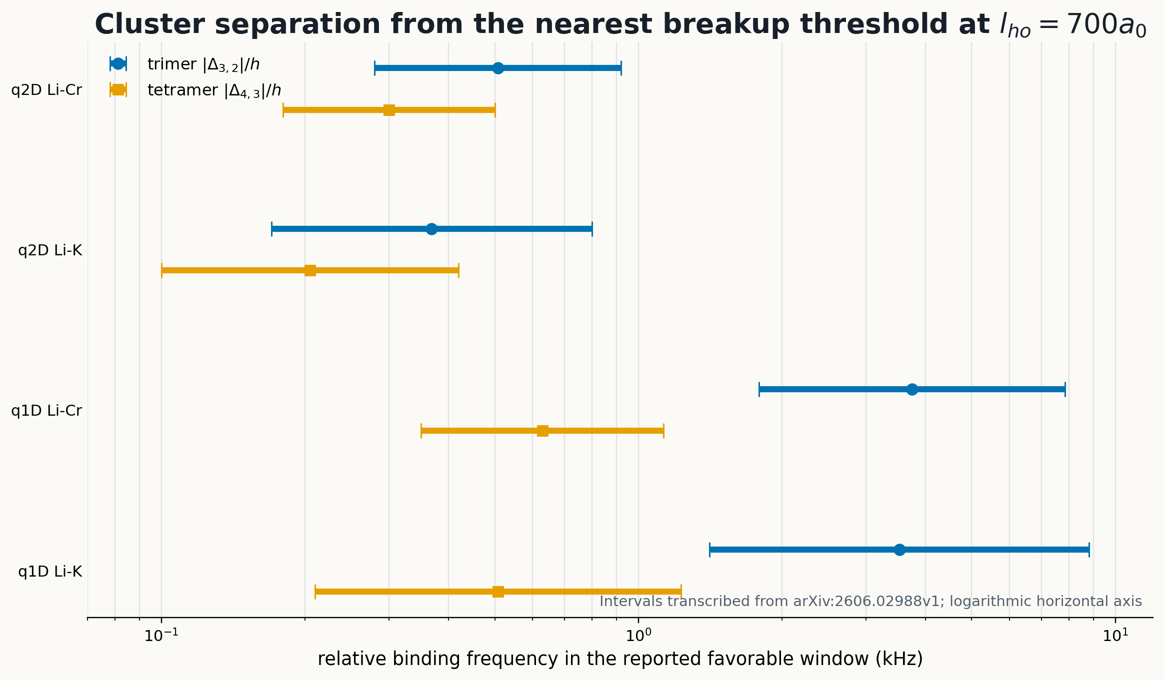
For Li–Cr, the favorable interval moves to $R^{\ast }/a_s\in (-194.0,-127.1)$ and gives

For Li–K, $R^{\ast }/a_s\in (-53.3,-25.7)$ gives

The deepest trimer separation anywhere on the plotted curves reaches $-8.10\mathrm{kHz}$ for Li–Cr and $-10.61\mathrm{kHz}$ for Li–K in quasi one dimension, compared with roughly $-0.92$ and $-0.97\mathrm{kHz}$ in quasi two dimensions. The tetramer gains absolute binding as well, while its ratio to the dimer scale can be smaller in quasi one dimension. The trimer receives the clearest spectroscopic advantage.

Figure 4. Magnitudes of the relative binding intervals quoted by Shi and Cui for $l_{\mathrm{ho}}=700a_0$. The horizontal axis is logarithmic. The blue trimer intervals move by roughly one decade between q2D and q1D. Tetramer intervals remain closer to the sub-kilohertz scale.

17. Multiple confinement-induced resonances

The calculated $a_{2\mathrm{D}}$ and $g_{1\mathrm{D}}=-(\mu a_{1\mathrm{D}}{)}^{-1}$ show several resonances as $R^{\ast }/a_s$ is scanned. Equal-frequency confinement would organize the two-body problem into a conserved center-of-mass quantum number. Species-selective confinement mixes those sectors, so several molecular center-of-mass levels acquire overlap with the open channel. Each dressed closed-channel level can cross threshold and generate a resonance.

The molecular-basis expression makes the mechanism explicit. A pole becomes strong when an eigenvalue $\mu /(2\pi a_s)+{\lambda }_j$ approaches zero and the corresponding eigenvector has a nonzero projected overlap $\sum _N{c}_{jN}{F}_{N;0,0}$. A zero eigenvalue with vanishing overlap would remain dark to the chosen incident channel. Resonance count and visibility therefore depend on both the spectrum and the contact overlap.

The effective range varies more smoothly than the scattering length across much of the negative-$a_s$ regime. Narrow resonances and tight confinement amplify its contribution. Fitting a single scattering length across adjacent resonances would merge physically distinct center-of-mass channels into a misleading parameter.

18. Reconstructing the confined-scattering and STM code

The second paper’s Figshare archive contains spreadsheets for Figs. 1–4 and no solver. A clean implementation should separate the confined two-body problem from the effective few-body problem.

18.1 Confined two-body module

The first module generates harmonic oscillator energies and normalized basis functions for each species and for the artificial molecule. It evaluates $F_{N;n_h,n_l}$ analytically where possible and by quadrature otherwise. Selection rules should be applied before numerical integration.

The second module evaluates ${\mathcal{M}}_{N{N}^{\prime }}(E,q)$. It treats short imaginary time with the analytic expansion, integrates the finite interval with adaptive quadrature, and handles the long-time open-channel subtraction separately. Tests should vary $t_0$ and any long-time split $t_c$. The final matrix must remain Hermitian below threshold.

The third module projects ${\mathcal{M}}^{-1}$ onto the open channel. It samples several momenta $q$ satisfying $q^2/(2\mu )\ll min({\omega }_h,{\omega }_l)$ and fits the inverse amplitude. The fit should include a diagnostic $q^4$ term even if only $a$ and $R$ are retained. Stability under removal of the largest-$q$ point gives a direct estimate of threshold-truncation error.

The fourth module searches for the exact confined dimer pole by tracking the lowest eigenvalue of $\mathcal{M}(E,0)$. The effective pole equation supplies an independent root. Storing both roots for every field and confinement value prevents a few hand-selected points from hiding a systematic drift.

for control in control_grid:
    a3d = scattering_length(control)

    def collision_matrix(E, q, n_cm):
        finite_propagator = regularized_imaginary_time_kernel(
            E=E,
            q=q,
            n_cm=n_cm,
            masses=masses,
            frequencies=frequencies,
            short_time_cut=t0,
        )
        inverse_contact = energy_dependent_inverse_scattering_length(
            E, a3d, R_star, reduced_mass
        )
        return inverse_contact * np.eye(n_cm) - finite_propagator

    inverse_t = []
    for q in threshold_momenta:
        M = collision_matrix(open_energy(q), q, n_cm)
        inverse_t.append(1 / project_open_channel(np.linalg.inv(M)))

    a_lowd, R_lowd, q4_diagnostic = fit_threshold_series(
        threshold_momenta, inverse_t
    )
    E2_exact = root_lowest_eigenvalue(collision_matrix, bracket=bound_window)
    E2_effective = root_effective_pole(a_lowd, R_lowd, geometry)

18.2 STM module

The STM solver takes only masses, geometry, $a$, and $R$ from the two-body stage. In quasi two dimensions, rotational decomposition converts angular dependence into Fourier channels. In quasi one dimension, the spectator momenta are signed scalars. A logarithmic or mapped momentum grid resolves both the shallow tail and the ultraviolet decay.

The trimer amplitude depends on one spectator momentum; the tetramer amplitude depends on two. Antisymmetry can be imposed by storing an ordered region and generating exchanged values with signs. Matrix-free Arnoldi iteration avoids constructing a dense tetramer kernel. For a trial $E<0$, the largest relevant eigenvalue ${\lambda }_{max}(E)$ is computed; a bound state satisfies ${\lambda }_{max}(E)=1$.

The momentum cutoff must be varied. In a properly universal calculation with finite effective range, the energy should stabilize before the cutoff reaches scales where the low-dimensional threshold expansion fails. Residual cutoff drift can indicate a missing higher-order shape parameter or an unresolved few-body counterterm.

18.3 Minimum convergence record

A complete numerical record would report the molecular center-of-mass cutoff, the single-particle oscillator cutoff, $t_0$, $t_c$, time-quadrature tolerance, threshold-fit interval, STM momentum cutoff, radial grid size, angular channel cutoff, and eigensolver tolerance. It would list $a_d$, $R_d$, $E_2^{\mathrm{exact}}$, $E_2^{\mathrm{effective}}$, $E_3$, and $E_4$ in the same table. The paper provides the physical curves and analytic regularization, but not this full convergence ledger.

19. What the two calculations have in common

Stage	Microwave-shielded molecules	Species-selective heteronuclear atoms
High-dimensional input	Anisotropic dressed $C_3/r^3+C_6/r^6$ interaction in free 3D	3D contact interaction, finite $R^{\ast }$, and two harmonic traps
Eliminated motion	Angular excursions from the attractive axis	Transverse oscillators and molecular COM channels
Retained low-energy object	Coordinate-space potentials $U^{(2)}$ and $U^{(3)}$	Threshold amplitudes described by $a_d$ and $R_d$
Direct benchmark	Exact 3D two-molecule partial-wave calculation	Exact confined two-body $T$-matrix pole
Few-body solver	Two-dimensional Jacobi grid for three identical molecules	q1D/q2D STM equations for $1+2$ and $1+3$ atoms
Statistics	Girardeau sign map between impenetrable bosons and fermions	Explicit antisymmetry under heavy-fermion exchange
Main extrapolation	Three molecules to a large crystalline chain	Two-body threshold fit to deeper three- and four-body kernels

The common structure is a sequence of controlled compressions. Both papers identify a low subspace, calculate the influence of excluded motion, test the reduction in a two-body observable, and solve a harder few-body problem with the reduced description. The discarded variables return as operators: a zero-point potential in one case, an energy-dependent scattering kernel in the other.

Figure 5. Evidence map for the two papers. “Exact” refers to exact diagonalization within the stated microscopic or confined model and numerical cutoffs. Each move to the right adds an effective-theory assumption. The labels prevent a two-body benchmark from being misreported as a full high-dimensional three- or four-body calculation.

20. Three meanings of universality

The molecular states have long-range universality. Their compact scale is set by $l_{\mathrm{\Omega }}$ inside a potential whose coefficients follow from $d$, $\mathrm{\Omega }$, and ${\delta }_r$. The repulsive core prevents access to chemistry, so no separate short-range boundary condition appears in the reduced model. Polarization remains an essential dimensionless parameter.

The heteronuclear clusters have scattering universality. The confined two-body dynamics are compressed into $a_{1\mathrm{D}/2\mathrm{D}}$ and $R_{1\mathrm{D}/2\mathrm{D}}$, after which the STM equations discard the microscopic Feshbach potential. This reduction remains quantitative only while the cluster kernel samples energies where the two-parameter threshold expansion is accurate.

The Bose–Fermi correspondence has kinematic universality. Once coincidence nodes divide a one-dimensional configuration space into ordered sectors, the energy-density mapping follows without using the detailed shape of the core. Finite transverse width and finite barrier penetration control the correction.

These meanings overlap, but they answer different questions. Long-range universality concerns sensitivity to chemical separation. Scattering universality concerns the number of low-energy constants. Kinematic universality concerns the topology of accessible configuration space.

21. Evidence audit and unresolved errors

The molecular paper gives its strongest evidence for two molecules. The exact three-dimensional calculation, the effective energy, the reduced-wavefunction overlap, and $G_2$ all agree over a quantified coupling range. The Born–Oppenheimer problem supplies a second high-dimensional check for one light and two infinitely heavy molecules. The equal-mass three-molecule spectrum is calculated only after the one-dimensional reduction.

The heteronuclear paper gives its strongest evidence for confined two-body scattering. It derives the UV-finite matrix and compares the effective pole with the exact confined pole. The trimer and tetramer energies come from low-dimensional STM equations. The paper does not present a full confined three- or four-body calculation.

The first paper neglects higher angular orders and interchannel derivative couplings. It adopts an analytic dressed potential at $\xi =\pi /4$ by extrapolation. It does not compute cluster lifetimes. Its large-$N$ droplet argument uses localized pair products and a dipolar tail estimate.

The second paper truncates the low-energy amplitude at $q^2$, provides no explicit cluster error bars, and does not report lifetime, finite-temperature, trap-anharmonicity, or preparation calculations. Its numerical examples use equal oscillator lengths even though the formalism permits arbitrary frequencies. The v1 text also contains editorial residues: the introduction mentions Li–Cs where the results use Li–Cr, and the q1D captions for Figs. 3 and 4 refer to an “effective 2D model.” The formulas and surrounding discussion identify those captions as typographical errors.

22. Public data and reproducibility

The first archive is roughly $30\mathrm{MB}$ and contains CSV/XLSX files, README descriptions, $1001\times 1001$ potential grids, two-dimensional wavefunction arrays, three-body potential surfaces, energies, overlaps, and Born–Oppenheimer curves. A reader can redraw the main plots and inspect the released arrays. Reconstructing the partial-wave Hamiltonian or the angular Hessian still requires new code.

The second archive is roughly $0.31\mathrm{MB}$ and contains spreadsheets for Figs. 1–4. It records scattering parameters and binding curves. It does not expose the imaginary-time integrator, basis cutoffs, fit windows, or STM eigensolver.

The distinction between plot reproducibility and computational reproducibility matters here. Plot reproducibility checks transcription and presentation. End-to-end reproduction tests the Hamiltonian, regularization, truncation, and convergence. Both archives support the first task and part of the second; neither supplies the complete executable pipeline.

23. Experimental decision points

The molecular proposal needs a joint map of binding and loss as polarization changes. The ideal point maximizes the ratio of binding energy to decay width, not the binding energy alone. A useful calculation would combine the effective axial state with a coupled-channel estimate of short-range flux for several $\xi <\pi /4$. Three-molecule spectroscopy should search below the two-molecule-plus-molecule threshold and compare bosonic and fermionic isotopologues at matched $l_d$ and $l_{\mathrm{\Omega }}$.

The heteronuclear proposal needs threshold resolution. Radio-frequency or modulation spectroscopy must resolve $|{\mathrm{\Delta }}_{3,2}|$ or $|{\mathrm{\Delta }}_{4,3}|$, rather than the total binding from free atoms. The q1D trimer windows are the strongest targets because their separations reach several kilohertz and retain ratios near twenty percent. Tetramers sit much closer to the trimer threshold, so temperature and loss broadening can erase them even when their absolute binding is substantial.

Trap calibration enters as a theoretical parameter, not a technical afterthought. A fractional error in either frequency changes the center-of-mass mixing, shifts every confinement-induced resonance, and modifies the fitted effective range. Anharmonicity can couple additional center-of-mass levels that are absent in the harmonic calculation.

24. Derivation check: the $r^{-4}$ core

Take an angular coordinate $\alpha$ with moment of inertia $I\sim m{r}^2$ and curvature

The zero-point energy scales as

When the $C_3$ curvature dominates, $E_{\mathrm{zp}}\propto r^{-5/2}$. When the $C_6$ curvature dominates, $E_{\mathrm{zp}}\propto r^{-4}$. The second power outruns the axial $-r^{-3}$ attraction and guarantees a short-distance turn upward within the quadratic regime.

Check the coefficient of the asymptotic minimum

Use

$$U(r)=-4C_3{r}^{-3}+4\hslash \sqrt{C_6/m}{r}^{-4}.$$Copy LaTeX

Then

$$\frac{dU}{dr}=12C_3{r}^{-4}-16\hslash \sqrt{C_6/m}{r}^{-5}=0,$$Copy LaTeX

which gives $r_m=4\hslash \sqrt{C_6/m}/(3C_3)$. Substitution of the published $C_3$ and $C_6$ yields $4\sqrt{2}(1+{\delta }_r^2{)}^{1/4}{l}_{\mathrm{\Omega }}$.

25. Derivation check: the center-of-mass cross term

Insert

into $m_h{\omega }_h^2{z}_h^2/2+m_l{\omega }_l^2{z}_l^2/2$. The coefficient of $Zz$ is

Equal oscillator length imposes $m_h{\omega }_h=m_l{\omega }_l$. For unequal masses, this relation guarantees unequal frequencies, so the cross term remains. The paper’s experimentally natural example therefore produces strong center-of-mass mixing.

26. Derivation check: total binding versus threshold separation

Consider $E_2=-10\mathrm{kHz}$, $E_3=-12\mathrm{kHz}$, and $E_4=-12.3\mathrm{kHz}$. The trimer separation is

while the tetramer separation is

The tetramer has the lowest total energy, yet its dissociation line sits only $0.3\mathrm{kHz}$ below the trimer threshold, equivalent to about $14\mathrm{nK}$. A spectrum can resolve the trimer and miss the tetramer.

27. A falsifiable reproduction program

A high-value reproduction would select three parameter points from each paper. For the molecular problem, one point should lie near the $s$-wave threshold, one near $\hslash \mathrm{\Omega }/E_u=10$, and one near 52. At each point, it should report exact even- and odd-parity energies, the effective energy, reduced-wavefunction overlap, angular width, and convergence with ${\ell }_{max}$. Those observables expose the crossover from three-dimensional threshold physics to the compact dual regime.

For the confined mixture, one point should lie far from a COM resonance, one on its flank, and one between adjacent resonances. Each point should report $a_d$, $R_d$, the $q^4$ coefficient, exact and effective dimer roots, and the maximum pair momentum sampled by the trimer and tetramer eigenvectors. Those data quantify whether the STM calculation remains inside the threshold-fit window.

The decisive extension for the first paper is a full three-dimensional equal-mass three-molecule calculation at one or two compact-state points. The decisive extension for the second is a confined three-body calculation at one q1D trimer point. Either benchmark would turn the present effective-theory evidence ladder into a closed high-dimensional loop.

28. Source trail

The two target preprints and their supplements are arXiv:2504.21535v4 and arXiv:2606.02988v1. Their data are available through Figshare 29306735 and Figshare 32507691.

The experimental field-linked tetramer result is X.-Y. Chen and collaborators, Nature 626, 283–287 (2024). Microwave shielding and its polarization dependence are treated by Karman and Hutson in PRL 121, 163401 and PRA 100, 052704. A recent scaling analysis of shielding universality is Dutta, Mukherjee, and Hutson, Physical Review Research 7, 023164.

The one-dimensional hard-core mapping originates with Girardeau, Journal of Mathematical Physics 1, 516 (1960). The confinement-induced resonance background is provided by Olshanii (1998) and Bergeman, Moore, and Olshanii (2003). The immediate quasi-two-dimensional cluster predecessor is Liu, Shi, Zaccanti, and Cui, Physical Review Research 6, L042004 (2024).

29. Final synthesis

The first paper finds a route to effective one-dimensional few-body physics without an external waveguide. The anisotropic microwave potential supplies the axis, and quantized angular motion supplies the core. Exact two-molecule calculations show where this reduction works and where three-dimensional threshold laws recover control. The three-molecule calculation then predicts a compact chain state, a Girardeau-type energy-density duality, and an extensive attractive correction for larger chains.

The second paper solves the two-body problem that an external waveguide creates when it traps two species differently. Center-of-mass and relative motion mix, several closed molecular levels become visible to the open channel, and a narrow Feshbach resonance leaves a large energy dependence. The authors retain that information in $a_d$ and $R_d$, verify the dimer pole, and predict q1D and q2D trimers and tetramers with STM equations. The strongest experimental window belongs to q1D trimers under tight confinement.

The calculations support a precise reading rule. Identify the high-dimensional benchmark, write down the information retained after projection, and mark every later result that uses the reduced object outside the benchmarked sector. Applied here, that rule leaves two substantial results intact: an interaction-generated one-dimensional molecular core with Bose–Fermi energy-density duality, and a finite-range, center-of-mass-coupled scattering theory that places heteronuclear clusters in experimentally measurable frequency windows.